What exactly is universal approximation about?

If you have read of neural networks, there’s some chance you must have heard of the universal approximation theorem. The key principle that makes these machines so powerful.

Universal Approximation Theorem

The Universal Approximation Theorem states that a feedforward neural network with a single hidden layer containing a finite number of neurons can approximate any continuous function on a compact subset of \(\mathbb{R}^n\), provided the activation function is non-constant, bounded, and continuous.

Formally:

Let \(K \subset \mathbb{R}\) be a compact set and \( f: K \to \mathbb{R} \) be a continuous function. For any \( \epsilon > 0 \), there exists a feedforward neural network \( g(x) \) of the form:

$$ g(x) = \sum_{i=1}^m c_i * a(w_i^\top x + b_i), $$

where:

- \( a: \mathbb{R} \to \mathbb{R} \) is the activation function,

- \( m \) is the number of neurons in the hidden layer,

- \( c_i \in \mathbb{R} \), \( w_i \in \mathbb{R} \), and \( b_i \in \mathbb{R} \) are parameters of the network,

such that:

$$ \sup_{x \in K} |f(x) - g(x)| < \epsilon. $$

This demonstrates that the network \( g(x) \) can approximate \( f(x) \) to arbitrary precision, given sufficient neurons in the hidden layer.

Uhhhhh WHAT?

To understand what the above theorem means, we will consider a simple neural network with a simple activation and assume that we are trying to approximate a one-dimensional function.

But before anything, we will get some definitions sorted first.

1. Approximation function

Let's call the function to be approximated as \( f(x) : \mathbb{R} \to \mathbb{R} \) and the approximating function as \( \hat{f}(x) : \mathbb{R} \to \mathbb{R} \)

2. Activation Function

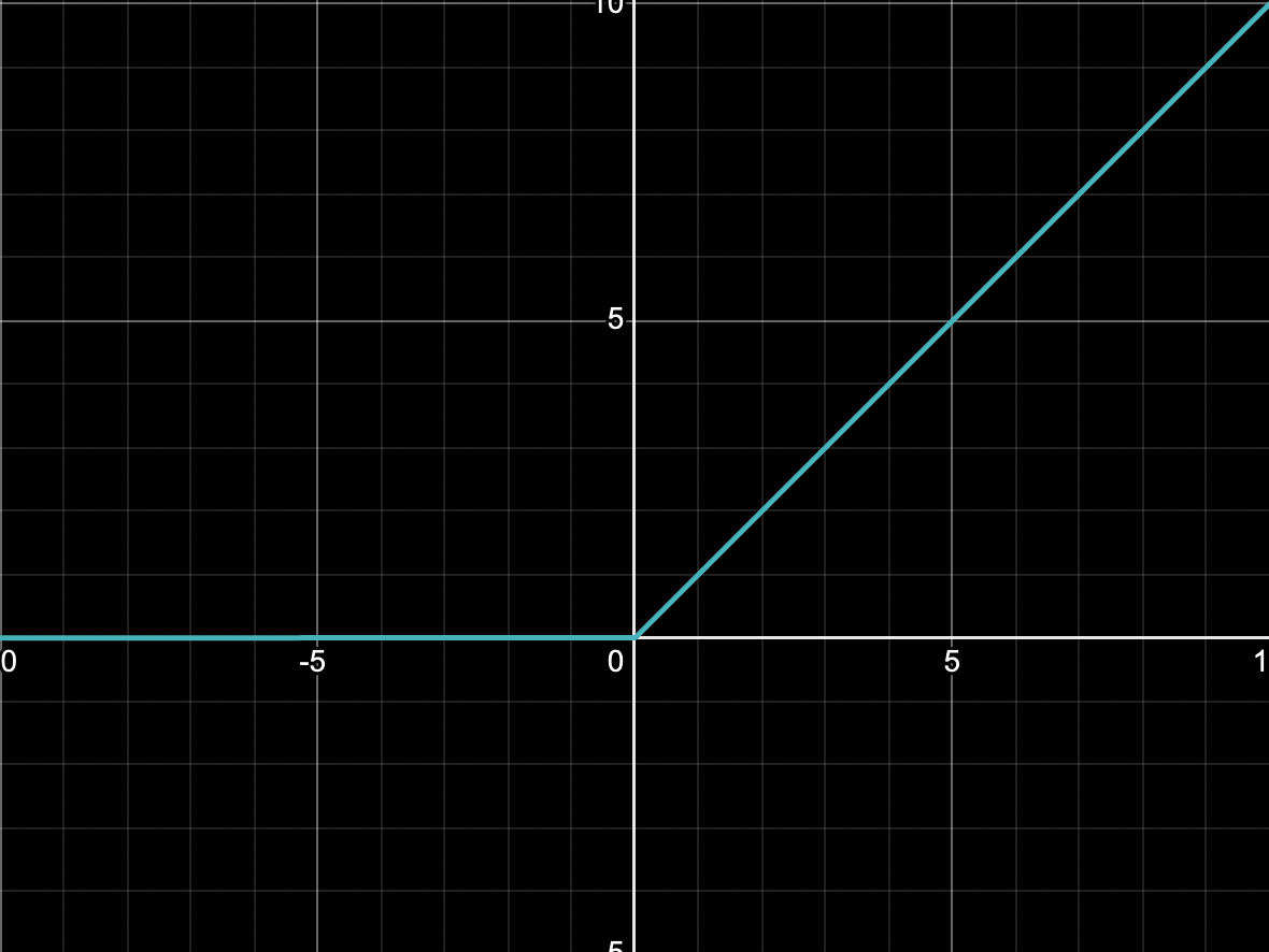
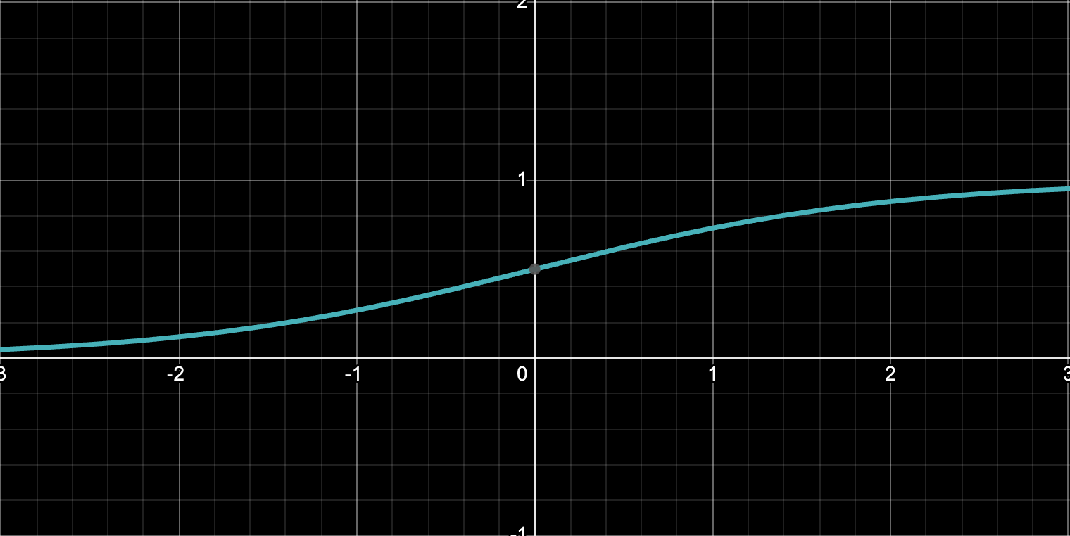
Basically, any non-linear function that transforms the input. Some most common ones with their graphs are:

- Rectified Linear Unit (ReLU) : \( \max(x, 0) \)

- Sigmoid : \( \frac{1}{1 + \exp(-x)} \)

3. Neural Network

Basically a summation of functions over and over again.

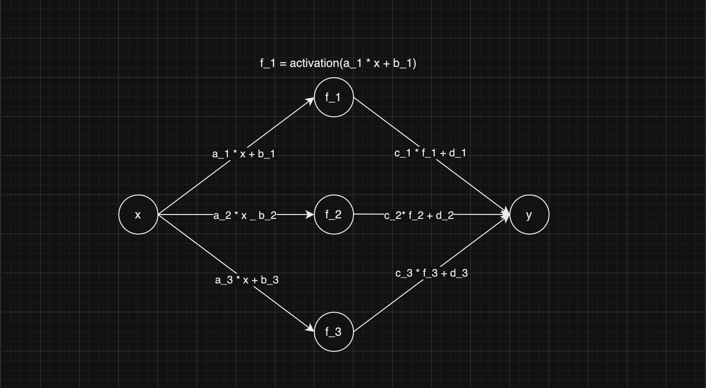
The neural network described in the image works as follows:

• Takes a single input (x) and sends it to the three nodes.
• Each of those nodes first maps this input to a different space using a linear function of the form (a*x + b).
• At each node, a non-linear activation function is applied to the mapped input and passed to the next layer.
• In the above diagram, the next layer just takes a summation of the outputs of all the three nodes, and that is the output of the neural network. When relevant parameters are learned, that is the approximated function.

A slightly more complicated neural network is described below:

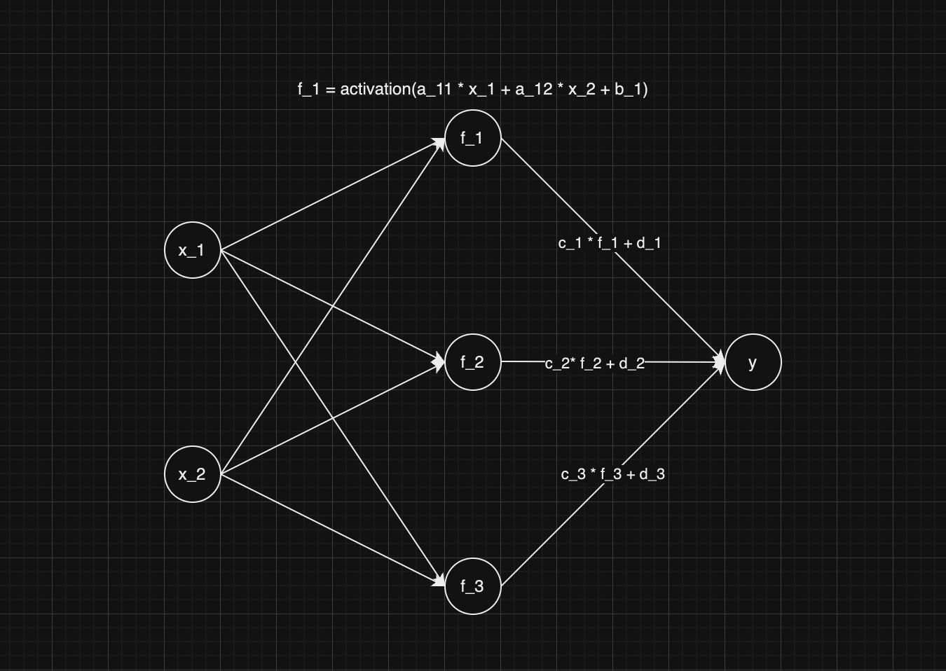
In this network, the hidden units again perform the same steps as above, but this time the linear function has two input parameters. We can extend this format for any dimension of input.

To sort of complete things, here is another type of neural network:

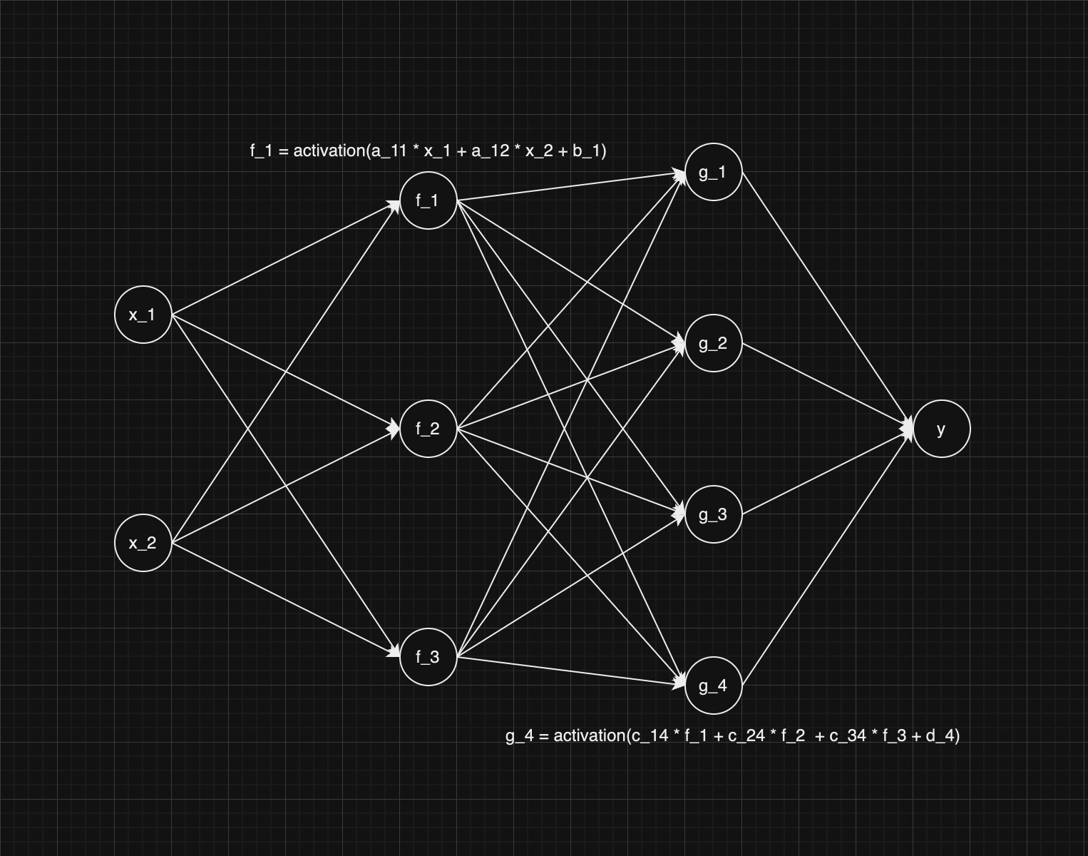
What you see above is a multiple-layer network. You can think of this recursively: the outputs from the first layer ((f_i)) become the inputs to the second layer. This recursive definition can be used to define any neural network of arbitrary depth.

You might have heard of multiple-layer neural networks performing exceptionally powerfully, but in theory, we can approximate any function using just a single hidden layer.

4. Piecewise Linear Functions

The final piece that we will require in this demo is the concept of a piecewise linear function. Let’s look at some graphs to understand them:

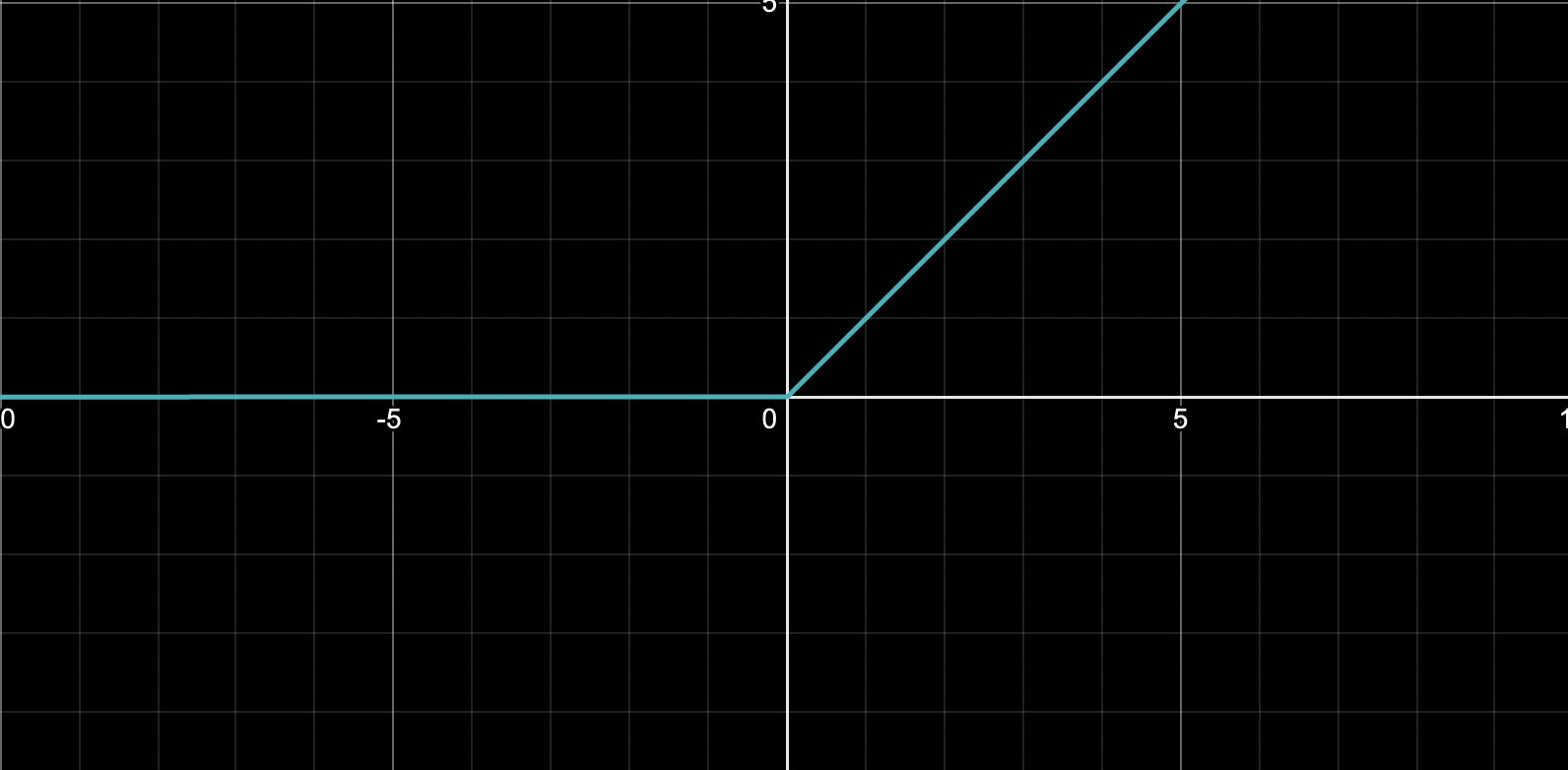
The above function is a basic ReLU function. As you can see, in the two regions where it’s differentiable, the function is linear. This is called piecewise linearity.

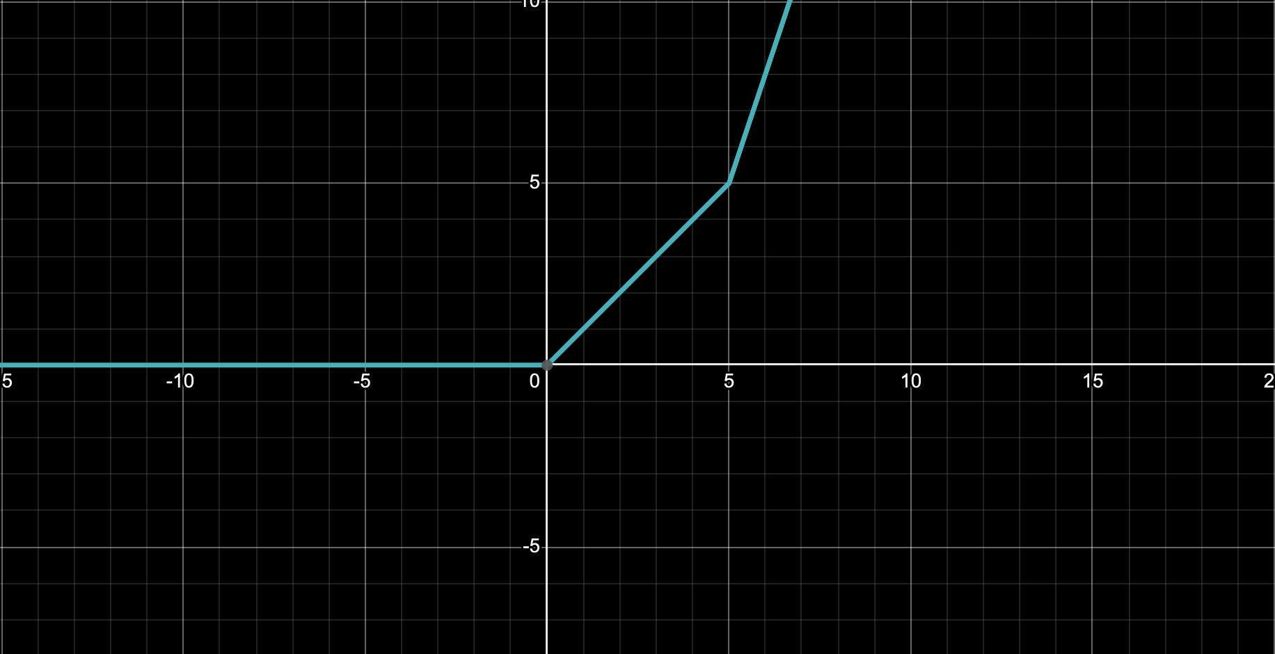
This one has three linear regions.

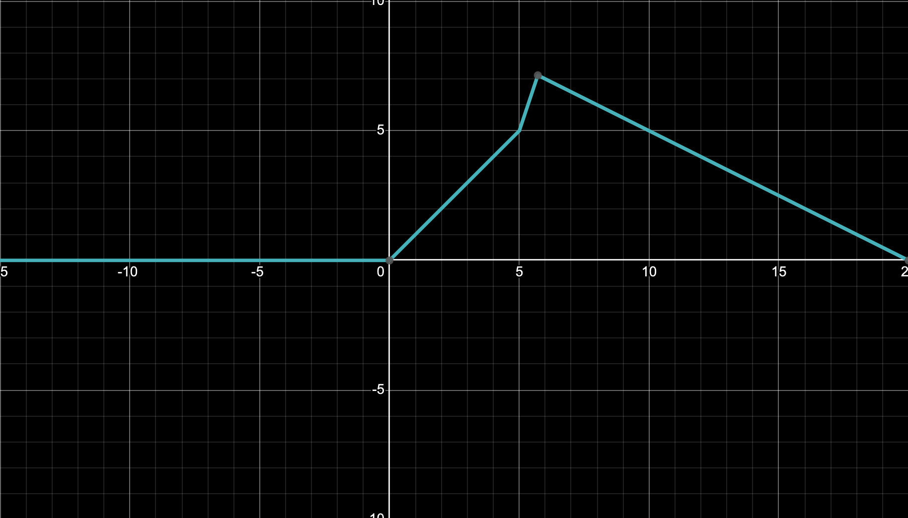
This one has four linear regions. All the graphs have been made by summing different ReLU functions. So you can see that adding ReLU basically gives a piecewise linear function.

With these basic definitions, let’s look at the universal approximation theorem.

Universal Approximation - A Visualization

In this visualization of the theorem, we will be approximating a very basic quadratic function (just (x^2)) using a single hidden layer neural network, and the activation we will be using here will be ReLU. We will vary the number of hidden units and look at the results of the approximation. The learning of the weights will be performed using the backpropagation algorithm, and the visualization will be done using matplotlib.

If \(N\) is the number of hidden units, the form of the approximation by a single hidden layer network can be written as:

$$ \hat{f}(x) = \sum_{i=1}^N c_i * ReLU(a_i * x + b_i) $$

Where \(a_i, b_i\), and \(c_i\) are constants that will be learned by the backpropagation algorithm by minimizing a certain loss function.

We will not go into the backpropagation algorithm in this blog, so we will just assume that the weights returned by backprop are optimal.

Summing ReLUs

The first thing we will try here is to show how summing up ReLUs can potentially approximate a quadratic curve.

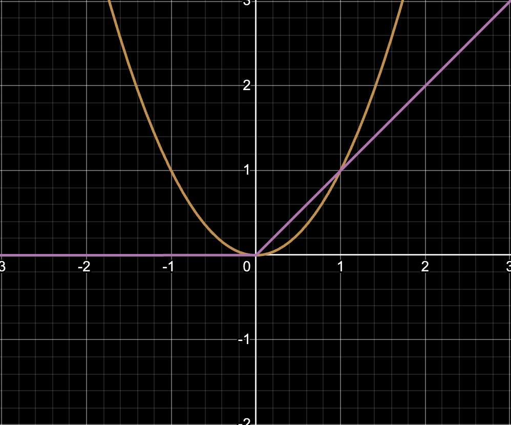
In the above figure, we have plotted \(y = x^2\) and \(ReLU(x)\). As you can observe, the approximation is pretty terrible here, and there are just two points where our approximation function hits the quadratic curve. However, this serves as a good starting point for us to understand how we can approximate functions using the universal approximation theorem.

Next, we will add one more ReLU function, and we will do it a little smartly. We will add it in such a way that the resulting piecewise continuous function comes closer to the right side of the quadratic curve.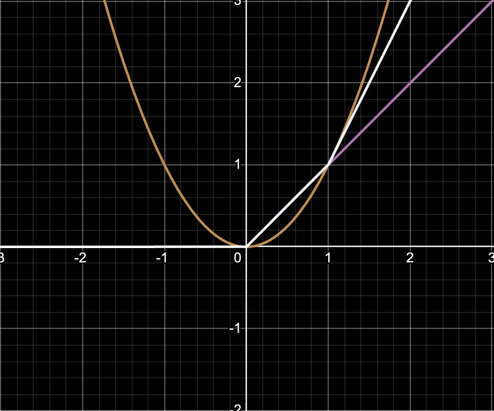

In the above graph, we have added (ReLU(x - 1)). The idea behind this was that the slope at (x = 1) is 2, and we want to ensure that the curve aligns better.

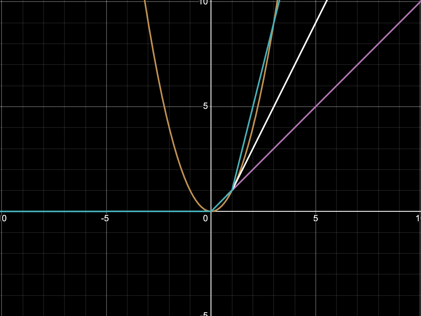
Now we do a symmetric addition of (ReLU(-x + 1)) to the function. This will ensure that the curve aligns better on the left side.

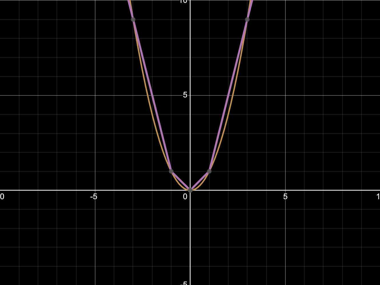
As you can observe the curve is now much closer to the quadratic curve. We can keep adding ReLU functions to get closer to the curve. The more ReLU functions we add, the closer we get to the curve.

Varying the number of hidden units - Animation

We will now look at how the approximation changes as we vary the number of hidden units. We will be using the same quadratic function and ReLU activation function. We will also be looking at the area under the curve of the difference between the approximated function and the quadratic function in the domain [-2,2] to understand how the approximation is improving.

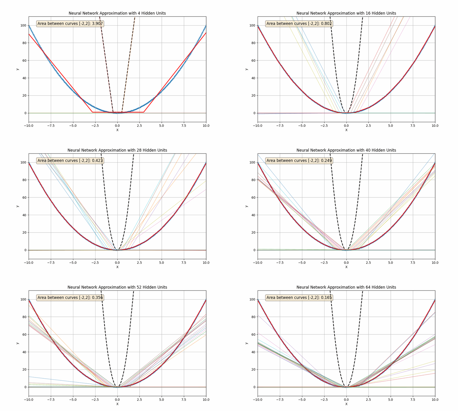
As you can observe in the above animation, the approximation gets better as we increase the number of hidden units. The area under the curve of the difference between the approximated function and the quadratic function decreases as we increase the number of hidden units.

With this demonstration, we can now move onto the proof of the universal approximation theorem.

Proof of the Universal Approximation Theorem for 1D Case

We are going to look at a special case of Universal Approximation using a Shallow Neural Network. We will be approximation univariate functions with univariate inputs.

Let \(sigma: \mathbb{R} \to \mathbb{R}\) be a continuous, non-constant, and sigmoidal activation function.

A standard example of a sigmoidal function is one satisfying \( lim_{x \to -\infty} \) \(sigma(x) = 0 \) and \( lim_{x \to +\infty} \sigma(x) = 1.\)

Then for any continuous function \(f: [a,b]\to \mathbb{R} \) and any \( \varepsilon > 0 \), there exist \(m \in \mathbb{N}\) and real coefficients \( v_0,,v_i,w_i ,b_i\) \( 1 \le i \le m\) such that

$$ \max_{x \in [a,b]} \Bigl|f(x) -\Bigl[v_0+\sum_{i=1}^{m} v_i \sigma\bigl(w_ix + b_i\bigr)\Bigr]\Bigr|<\varepsilon $$

In other words, single-hidden-layer neural networks with a sigmoidal activation can uniformly approximate any continuous function on a compact interval as closely as we want.

We build the proof in several phases:

1. Show that \( \sigma(\alpha(x - t)) \) approximates a step function.

2. Use step functions to approximate continuous functions by piecewise constants.

3. Replace exact step functions in the piecewise-constant approximation with sigmoidal “smoothed” steps.
4. Combine the two approximations to control the overall error.

Phase 1 - Sigmoid Approximates Step Function

Define the Heaviside (unit) step function \( H : \mathbb{R} \to \{0, 1\} \) by

$$ H(u) = \begin{cases} 0, & u < 0, \\ 1, & u \geq 0. \end{cases} $$

A key property of a sigmoidal \( \sigma \) is:

$$ \lim_{z \to -\infty} \sigma(z) = 0, \quad \lim_{z \to +\infty} \sigma(z) = 1. $$

Given any \( \delta > 0 \) and a bounded interval \([A, B] \subset \mathbb{R}\), there exists a sufficiently large scalar \( \alpha > 0 \) (depending on \( \delta \) and \([A, B]\)) such that, for every \( x \in [A, B] \),

$$ \lvert \sigma(\alpha x) - H(x) \rvert < \delta. $$

Intuitively, as \( \alpha \to \infty \), the graph of \( y = \sigma(\alpha x) \) becomes a steeper and steeper "S-curve" approximating the jump at \( 0 \).

If we want a "jump" around \( x = t \), we look at \( \sigma(\alpha(x - t)) \). For large \( \alpha \), this approximates

$$ x \mapsto H(x - t) = \begin{cases} 0, & x < t, \\ 1, & x \geq t. \end{cases} $$

We can make

$$ \max_{x \in [a, b]} \lvert \sigma(\alpha(x - t)) - H(x - t) \rvert $$

arbitrarily small by choosing \( \alpha \) large enough (the choice depends on how large \([a, b]\) is and on \( \delta \)).

Phase 2.1 - Piecewise Constant Approximation

By the uniform continuity of \( f \) on the compact interval \([a, b]\), for any \( \epsilon > 0 \), there is a partition of \([a, b]\):

\( a = x_0 < x_1 < x_2 < .... < x_{N-1} < x_N = b \)

so that on each subinterval \([x_{k-1}, x_k]\), the oscillation of \( f \) is at most \( \epsilon / 2 \). Concretely, pick some point \( \xi_k \in [x_{k-1}, x_k] \) and let

\[ c_k = f(\xi_k). \]

Then define a piecewise-constant approximation \( F \) by

\[ F(x) = \sum_{k=1}^{N} c_k \cdot \mathbf{1}_{[x_{k-1}, x_k)}(x). \]

Equivalently,

$$ F(x) = \sum_{k=1}^{N} c_k \left[ H(x - x_{k-1}) - H(x - x_k) \right].$$

Each bracket is 1 precisely when \( x \in [x_{k-1}, x_k) \) and 0 otherwise. By construction,

$$ \max_{x \in [a, b]} \left| f(x) - F(x) \right| \leq \frac{\epsilon}{2}. $$

Phase 2.2 - How does Uniform Continuity help with the interval partition?

A standard result in real analysis is:

Heine–Cantor Theorem: If a function ( f ) is continuous on a compact set (here ([a, b])), then ( f ) is uniformly continuous.

Uniform continuity says:

For every \(\epsilon' > 0\), there exists a \(\delta > 0\) such that for all \( x, y\in [a, b]\), if \( |x - y| < \delta\) , then \(|f(x) - f(y)| < \epsilon'\).

We will choose \( \epsilon' := \frac{\epsilon}{2} \). So: Given \( \epsilon > 0 \), pick \( \delta > 0 \) such that for any \( x, y \) with \( |x - y| < \delta \), we have

$$ |f(x) - f(y)| < \frac{\epsilon}{2}. $$

That’s the key.

With this \( \delta > 0 \) in hand, we subdivide \([a, b]\) into \( N \) intervals so small that the maximum length of each subinterval is strictly less than \( \delta \). One standard way:

1. Choose \( N \) so that

$$ \frac{b - a}{N} < \delta. $$

2. Define the partition points:

$$ x_i = a + i \cdot \frac{b - a}{N}, \quad i = 0, 1, \ldots, N. $$

Then each subinterval \([x_{i-1}, x_i]\) has length

$$ \frac{b - a}{N}, $$

which is \( < \delta \).

Concretely,

$$ a = x_0 < x_1 < x_2 < \cdots < x_{N-1} < x_N = b, $$

with

$$ x_i - x_{i-1} = \frac{b - a}{N} < \delta. $$

Now, for any \( i = 1, \ldots, N \) and for any \( x, y \in [x_{i-1}, x_i] \), we have

$$ |x - y| \leq x_i - x_{i-1} = \frac{b - a}{N} < \delta. $$

Hence, by the choice of \( \delta \),

$$ |f(x) - f(y)| < \frac{\epsilon}{2}. $$

In other words, the function's oscillation on each subinterval \([x_{i-1}, x_i]\) is at most \( \frac{\epsilon}{2} \). Formally,

$$ \sup_{x, y \in [x_{i-1}, x_i]} |f(x) - f(y)| \leq \frac{\epsilon}{2}. $$

That’s exactly what we wanted to show.

Phase 3 - Sigmoid Again

Now, we replace the ideal step \( H(\cdot) \) by the approximate step \( \sigma(\alpha(\cdot)) \). Define

$$ F_\alpha(x) = \sum_{k=1}^N c_k \left[ \sigma\left(\alpha (x - x_{k-1})\right) - \sigma\left(\alpha (x - x_k)\right) \right] $$

Each term \( \sigma\left(\alpha (x - x_{k-1})\right) \) approximates \( H(x - x_{k-1}) \), and similarly for \( \sigma\left(\alpha (x - x_k)\right) \). As a result, for sufficiently large \( \alpha \):

$$ \left| F(x) - F_\alpha(x) \right| \le \sum_{k=1}^N c_k \left( \left [ H(x - x_{k-1}) - \sigma\left(\alpha (x - x_{k-1})\right) \right] - \left[\left( H(x - x_{k}) - \sigma\left(\alpha (x - x_k)\right) \right) \right] \right) $$

$$ \left| F(x) - F_\alpha(x) \right| \le \sum_{k=1}^N |c_k| \left| \left [ H(x - x_{k-1}) - \sigma\left(\alpha (x - x_{k-1})\right) \right] | + |\left( H(x - x_{k}) - \sigma\left(\alpha (x - x_k)\right) \right) \right)| $$

$$ \left| F(x) - F_\alpha(x) \right| \le 2N * \beta * |c_{max}| $$

where \( \beta \) can be arbitrarily selected and \( c_{max} \) is the maximum value of \( c_k \). We select beta such that the whole equation is less than \( \frac{\epsilon}{2} \).

Phase 4 - Combine the Errors

We already have

$$ \max_{x \in [a, b]} \lvert f(x) - F(x) \rvert \leq \frac{\epsilon}{2}. $$

Also, we have

$$ \max_{x \in [a, b]} \lvert F(x) - F_\alpha(x) \rvert \leq \frac{\epsilon}{2}. $$

By the triangle inequality,

$$ \max_{x \in [a, b]} \lvert f(x) - F_\alpha(x) \rvert \leq \max_{x \in [a, b]} \lvert f(x) - F(x) \rvert + \max_{x \in [a, b]} \lvert F(x) - F_\alpha(x) \rvert < \epsilon. $$

Thus, \( F_\alpha \) is within \( \epsilon \) of \( f \) uniformly on \([a, b]\).

Phase 5 - Expressing the approximation as a Single-Hidden-Layer Network

Recall:

$$ F_\alpha(x) = \sum_{k=1}^N c_k \left[ \sigma\left(\alpha (x - x_{k-1})\right) - \sigma\left(\alpha (x - x_k)\right) \right]. $$

Notice that each bracketed term is a linear combination of sigmoids \( \sigma(\alpha x + b) \) for some bias \( b \) (specifically, \( b = -\alpha x_{k-1} \) or \( b = -\alpha x_k \)). If we label each instance of \( \sigma(\cdot) \) as a "hidden neuron," then \( F_\alpha \) is exactly

$$ v_0 + \sum_{i=1}^{2N} v_i \sigma(w_i x + b_i), $$

where:

- \( 2N \) is the total count of sigmoids (two for each subinterval, though some proofs can combine them cleverly),

- \( w_i = \pm \alpha \), and

- \( v_i, b_i \) are real coefficients constructed from the \(\{c_k\}\) and the partition \(\{x_k\}\).

- \( v_0 \) may be \( 0 \) or another simple constant offset if needed.

Hence, the function \( F_\alpha \) is literally a single-hidden-layer neural network with a sigmoidal activation.

Putting it all together, we see that for any \( \epsilon > 0 \), we can find such an \( F_\alpha \) so that

$$ \max_{x \in [a, b]} \lvert f(x) - F_\alpha(x) \rvert < \epsilon. $$

This completes the proof that single-hidden-layer networks (with \( \sigma \) sigmoidal) can approximate continuous functions on a compact interval arbitrarily well.

In the above five phases of the proof, we have shown that a single-hidden-layer neural network with a sigmoidal activation function can approximate any continuous function on a compact interval as closely as we want. This is the essence of the Universal Approximation Theorem.

Conclusion

The Universal Approximation Theorem is a fundamental result in the theory of neural networks. It states that a feedforward neural network with a single hidden layer containing a finite number of neurons can approximate any continuous function on a compact subset of \(\mathbb{R}^n\), provided the activation function is non-constant, bounded, and continuous.

The theorem is a key principle that makes neural networks so powerful. It demonstrates that the network can approximate any function to arbitrary precision, given sufficient neurons in the hidden layer. This is the reason why neural networks are so widely used in machine learning and artificial intelligence.

There are proofs that generalize the proof the multi-dimensional case, but the essence remains the same. The theorem is a powerful tool that underpins the success of neural networks in a wide range of applications.

Proofs for other activation functions and deeper networks are also available, but the single-hidden-layer case is the most fundamental and widely used. You can refer to the original paper by Kurt Hornik for more details.

I hope this blog helped you understand the Universal Approximation Theorem better. If you have any questions or feedback, feel free to reach out to me. Thanks for reading!